Using R for Multivariate Analysis
Multivariate Analysis
This booklet tells you how to use the R statistical software to carry out some simple multivariate analyses, with a focus on principal components analysis (PCA) and linear discriminant analysis (LDA).
This booklet assumes that the reader has some basic knowledge of multivariate analyses, and the principal focus of the booklet is not to explain multivariate analyses, but rather to explain how to carry out these analyses using R.
If you are new to multivariate analysis, and want to learn more about any of the concepts presented here, I would highly recommend the Open University book “Multivariate Analysis” (product code M249/03), available from from the Open University Shop.
In the examples in this booklet, I will be using data sets from the UCI Machine Learning Repository, http://archive.ics.uci.edu/ml.
There is a pdf version of this booklet available at https://media.readthedocs.org/pdf/little-book-of-r-for-multivariate-analysis/latest/little-book-of-r-for-multivariate-analysis.pdf.
If you like this booklet, you may also like to check out my booklet on using R for biomedical statistics, http://a-little-book-of-r-for-biomedical-statistics.readthedocs.org/, and my booklet on using R for time series analysis, http://a-little-book-of-r-for-time-series.readthedocs.org/.
Reading Multivariate Analysis Data into R
The first thing that you will want to do to analyse your multivariate data will be to read it into R, and to plot the data. You can read data into R using the read.table() function.
For example, the file http://archive.ics.uci.edu/ml/machine-learning-databases/wine/wine.data contains data on concentrations of 13 different chemicals in wines grown in the same region in Italy that are derived from three different cultivars.
The data set looks like this:
1,14.23,1.71,2.43,15.6,127,2.8,3.06,.28,2.29,5.64,1.04,3.92,1065
1,13.2,1.78,2.14,11.2,100,2.65,2.76,.26,1.28,4.38,1.05,3.4,1050
1,13.16,2.36,2.67,18.6,101,2.8,3.24,.3,2.81,5.68,1.03,3.17,1185
1,14.37,1.95,2.5,16.8,113,3.85,3.49,.24,2.18,7.8,.86,3.45,1480
1,13.24,2.59,2.87,21,118,2.8,2.69,.39,1.82,4.32,1.04,2.93,735
...
There is one row per wine sample. The first column contains the cultivar of a wine sample (labelled 1, 2 or 3), and the following thirteen columns contain the concentrations of the 13 different chemicals in that sample. The columns are separated by commas.
When we read the file into R using the read.table() function, we need to use the “sep=” argument in read.table() to tell it that the columns are separated by commas. That is, we can read in the file using the read.table() function as follows:
> wine <- read.table("http://archive.ics.uci.edu/ml/machine-learning-databases/wine/wine.data",
          sep=",")
> wine
     V1    V2   V3   V4   V5  V6   V7   V8   V9  V10       V11   V12  V13  V14
 1    1 14.23 1.71 2.43 15.6 127 2.80 3.06 0.28 2.29  5.640000 1.040 3.92 1065
 2    1 13.20 1.78 2.14 11.2 100 2.65 2.76 0.26 1.28  4.380000 1.050 3.40 1050
 3    1 13.16 2.36 2.67 18.6 101 2.80 3.24 0.30 2.81  5.680000 1.030 3.17 1185
 4    1 14.37 1.95 2.50 16.8 113 3.85 3.49 0.24 2.18  7.800000 0.860 3.45 1480
 5    1 13.24 2.59 2.87 21.0 118 2.80 2.69 0.39 1.82  4.320000 1.040 2.93  735
 ...
 176  3 13.27 4.28 2.26 20.0 120 1.59 0.69 0.43 1.35 10.200000 0.590 1.56  835
 177  3 13.17 2.59 2.37 20.0 120 1.65 0.68 0.53 1.46  9.300000 0.600 1.62  840
 178  3 14.13 4.10 2.74 24.5  96 2.05 0.76 0.56 1.35  9.200000 0.610 1.60  560
In this case the data on 178 samples of wine has been read into the variable ‘wine’.
Plotting Multivariate Data
Once you have read a multivariate data set into R, the next step is usually to make a plot of the data.
A Matrix Scatterplot
One common way of plotting multivariate data is to make a “matrix scatterplot”, showing each pair of variables plotted against each other. We can use the “scatterplotMatrix()” function from the “car” R package to do this. To use this function, we first need to install the “car” R package (for instructions on how to install an R package, see How to install an R package).
Once you have installed the “car” R package, you can load the “car” R package by typing:
> library("car")
You can then use the “scatterplotMatrix()” function to plot the multivariate data.
To use the scatterplotMatrix() function, you need to give it as its input the variables that you want included in the plot. Say for example, that we just want to include the variables corresponding to the concentrations of the first five chemicals. These are stored in columns 2-6 of the variable “wine”. We can extract just these columns from the variable “wine” by typing:
> wine[2:6]
         V2   V3   V4   V5  V6
  1   14.23 1.71 2.43 15.6 127
  2   13.20 1.78 2.14 11.2 100
  3   13.16 2.36 2.67 18.6 101
  4   14.37 1.95 2.50 16.8 113
  5   13.24 2.59 2.87 21.0 118
  ...
To make a matrix scatterplot of just these 13 variables using the scatterplotMatrix() function we type:
> scatterplotMatrix(wine[2:6])
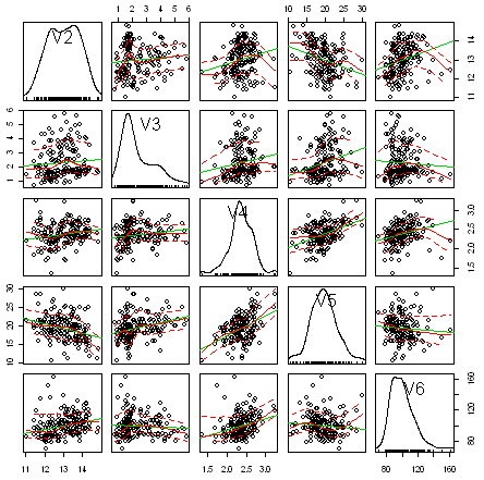
In this matrix scatterplot, the diagonal cells show histograms of each of the variables, in this case the concentrations of the first five chemicals (variables V2, V3, V4, V5, V6).
Each of the off-diagonal cells is a scatterplot of two of the five chemicals, for example, the second cell in the first row is a scatterplot of V2 (y-axis) against V3 (x-axis).
A Scatterplot with the Data Points Labelled by their Group
If you see an interesting scatterplot for two variables in the matrix scatterplot, you may want to plot that scatterplot in more detail, with the data points labelled by their group (their cultivar in this case).
For example, in the matrix scatterplot above, the cell in the third column of the fourth row down is a scatterplot of V5 (x-axis) against V4 (y-axis). If you look at this scatterplot, it appears that there may be a positive relationship between V5 and V4.
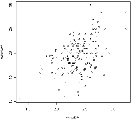
We may therefore decide to examine the relationship between V5 and V4 more closely, by plotting a scatterplot of these two variable, with the data points labelled by their group (their cultivar). To plot a scatterplot of two variables, we can use the “plot” R function. The V4 and V5 variables are stored in the columns V4 and V5 of the variable “wine”, so can be accessed by typing wine$V4 or wine$V5. Therefore, to plot the scatterplot, we type:
> plot(wine$V4, wine$V5)
If we want to label the data points by their group (the cultivar of wine here), we can use the “text” function in R to plot some text beside every data point. In this case, the cultivar of wine is stored in the column V1 of the variable “wine”, so we type:
> text(wine$V4, wine$V5, wine$V1, cex=0.7, pos=4, col="red")
If you look at the help page for the “text” function, you will see that “pos=4” will plot the text just to the right of the symbol for a data point. The “cex=0.5” option will plot the text at half the default size, and the “col=red” option will plot the text in red. This gives us the following plot:
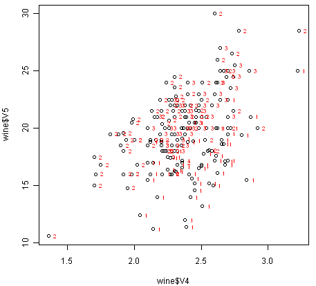
We can see from the scatterplot of V4 versus V5 that the wines from cultivar 2 seem to have lower values of V4 compared to the wines of cultivar 1.
A Profile Plot
Another type of plot that is useful is a “profile plot”, which shows the variation in each of the variables, by plotting the value of each of the variables for each of the samples.
The function “makeProfilePlot()” below can be used to make a profile plot. This function requires the “RColorBrewer” library. To use this function, we first need to install the “RColorBrewer” R package (for instructions on how to install an R package, see How to install an R package).
> makeProfilePlot <- function(mylist,names)
  {
     require(RColorBrewer)
     # find out how many variables we want to include
     numvariables <- length(mylist)
     # choose 'numvariables' random colours
     colours <- brewer.pal(numvariables,"Set1")
     # find out the minimum and maximum values of the variables:
     mymin <- 1e+20
     mymax <- 1e-20
     for (i in 1:numvariables)
     {
        vectori <- mylist[[i]]
        mini <- min(vectori)
        maxi <- max(vectori)
        if (mini < mymin) { mymin <- mini }
        if (maxi > mymax) { mymax <- maxi }
     }
     # plot the variables
     for (i in 1:numvariables)
     {
        vectori <- mylist[[i]]
        namei <- names[i]
        colouri <- colours[i]
        if (i == 1) { plot(vectori,col=colouri,type="l",ylim=c(mymin,mymax)) }
        else         { points(vectori, col=colouri,type="l")                                     }
        lastxval <- length(vectori)
        lastyval <- vectori[length(vectori)]
        text((lastxval-10),(lastyval),namei,col="black",cex=0.6)
     }
  }
To use this function, you first need to copy and paste it into R. The arguments to the function are a vector containing the names of the varibles that you want to plot, and a list variable containing the variables themselves.
For example, to make a profile plot of the concentrations of the first five chemicals in the wine samples (stored in columns V2, V3, V4, V5, V6 of variable “wine”), we type:
> library(RColorBrewer)
> names <- c("V2","V3","V4","V5","V6")
> mylist <- list(wine$V2,wine$V3,wine$V4,wine$V5,wine$V6)
> makeProfilePlot(mylist,names)
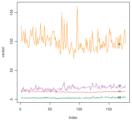
It is clear from the profile plot that the mean and standard deviation for V6 is quite a lot higher than that for the other variables.
Calculating Summary Statistics for Multivariate Data
Another thing that you are likely to want to do is to calculate summary statistics such as the mean and standard deviation for each of the variables in your multivariate data set.
This is easy to do, using the “mean()” and “sd()” functions in R. For example, say we want to calculate the mean and standard deviations of each of the 13 chemical concentrations in the wine samples. These are stored in columns 2-14 of the variable “wine”. So we type:
> sapply(wine[2:14],mean)
          V2          V3          V4          V5          V6          V7
  13.0006180   2.3363483   2.3665169  19.4949438  99.7415730   2.2951124
          V8          V9         V10         V11         V12         V13
   2.0292697   0.3618539   1.5908989   5.0580899   0.9574494   2.6116854
          V14
  746.8932584
This tells us that the mean of variable V2 is 13.0006180, the mean of V3 is 2.3363483, and so on.
Similarly, to get the standard deviations of the 13 chemical concentrations, we type:
> sapply(wine[2:14],sd)
          V2          V3          V4          V5          V6          V7
   0.8118265   1.1171461   0.2743440   3.3395638  14.2824835   0.6258510
          V8          V9         V10         V11         V12         V13
   0.9988587   0.1244533   0.5723589   2.3182859   0.2285716   0.7099904
          V14
   314.9074743
We can see here that it would make sense to standardise in order to compare the variables because the variables have very different standard deviations - the standard deviation of V14 is 314.9074743, while the standard deviation of V9 is just 0.1244533. Thus, in order to compare the variables, we need to standardise each variable so that it has a sample variance of 1 and sample mean of 0. We will explain below how to standardise the variables.
Means and Variances Per Group
It is often interesting to calculate the means and standard deviations for just the samples from a particular group, for example, for the wine samples from each cultivar. The cultivar is stored in the column “V1” of the variable “wine”.
To extract out the data for just cultivar 2, we can type:
> cultivar2wine <- wine[wine$V1=="2",]
We can then calculate the mean and standard deviations of the 13 chemicals’ concentrations, for just the cultivar 2 samples:
> sapply(cultivar2wine[2:14],mean)
    V2         V3         V4         V5         V6         V7         V8
  12.278732   1.932676   2.244789  20.238028  94.549296   2.258873   2.080845
    V9        V10        V11        V12        V13        V14
  0.363662   1.630282   3.086620   1.056282   2.785352 519.507042
> sapply(cultivar2wine[2:14])
    V2          V3          V4          V5          V6          V7          V8
  0.5379642   1.0155687   0.3154673   3.3497704  16.7534975   0.5453611   0.7057008
    V9         V10         V11         V12         V13         V14
  0.1239613   0.6020678   0.9249293   0.2029368   0.4965735 157.2112204
You can calculate the mean and standard deviation of the 13 chemicals’ concentrations for just cultivar 1 samples, or for just cultivar 3 samples, in a similar way.
However, for convenience, you might want to use the function “printMeanAndSdByGroup()” below, which prints out the mean and standard deviation of the variables for each group in your data set:
> printMeanAndSdByGroup <- function(variables,groupvariable)
  {
     # find the names of the variables
     variablenames <- c(names(groupvariable),names(as.data.frame(variables)))
     # within each group, find the mean of each variable
     groupvariable <- groupvariable[,1] # ensures groupvariable is not a list
     means <- aggregate(as.matrix(variables) ~ groupvariable, FUN = mean)
     names(means) <- variablenames
     print(paste("Means:"))
     print(means)
     # within each group, find the standard deviation of each variable:
     sds <- aggregate(as.matrix(variables) ~ groupvariable, FUN = sd)
     names(sds) <- variablenames
     print(paste("Standard deviations:"))
     print(sds)
     # within each group, find the number of samples:
     samplesizes <- aggregate(as.matrix(variables) ~ groupvariable, FUN = length)
     names(samplesizes) <- variablenames
     print(paste("Sample sizes:"))
     print(samplesizes)
  }
To use the function “printMeanAndSdByGroup()”, you first need to copy and paste it into R. The arguments of the function are the variables that you want to calculate means and standard deviations for, and the variable containing the group of each sample. For example, to calculate the mean and standard deviation for each of the 13 chemical concentrations, for each of the three different wine cultivars, we type:
> printMeanAndSdByGroup(wine[2:14],wine[1])
  [1] "Means:"
    V1       V2       V3       V4       V5       V6       V7        V8       V9      V10      V11       V12      V13       V14
  1  1 13.74475 2.010678 2.455593 17.03729 106.3390 2.840169 2.9823729 0.290000 1.899322 5.528305 1.0620339 3.157797 1115.7119
  2  2 12.27873 1.932676 2.244789 20.23803  94.5493 2.258873 2.0808451 0.363662 1.630282 3.086620 1.0562817 2.785352  519.5070
  3  3 13.15375 3.333750 2.437083 21.41667  99.3125 1.678750 0.7814583 0.447500 1.153542 7.396250 0.6827083 1.683542  629.8958
  [1] "Standard deviations:"
    V1        V2        V3        V4       V5       V6        V7        V8         V9       V10       V11       V12       V13      V14
  1  1 0.4621254 0.6885489 0.2271660 2.546322 10.49895 0.3389614 0.3974936 0.07004924 0.4121092 1.2385728 0.1164826 0.3570766 221.5208
  2  2 0.5379642 1.0155687 0.3154673 3.349770 16.75350 0.5453611 0.7057008 0.12396128 0.6020678 0.9249293 0.2029368 0.4965735 157.2112
  3  3 0.5302413 1.0879057 0.1846902 2.258161 10.89047 0.3569709 0.2935041 0.12413959 0.4088359 2.3109421 0.1144411 0.2721114 115.0970
  [1] "Sample sizes:"
    V1 V2 V3 V4 V5 V6 V7 V8 V9 V10 V11 V12 V13 V14
  1  1 59 59 59 59 59 59 59 59  59  59  59  59  59
  2  2 71 71 71 71 71 71 71 71  71  71  71  71  71
  3  3 48 48 48 48 48 48 48 48  48  48  48  48  48
The function “printMeanAndSdByGroup()” also prints out the number of samples in each group. In this case, we see that there are 59 samples of cultivar 1, 71 of cultivar 2, and 48 of cultivar 3.
Between-groups Variance and Within-groups Variance for a Variable
If we want to calculate the within-groups variance for a particular variable (for example, for a particular chemical’s concentration), we can use the function “calcWithinGroupsVariance()” below:
> calcWithinGroupsVariance <- function(variable,groupvariable)
  {
     # find out how many values the group variable can take
     groupvariable2 <- as.factor(groupvariable[[1]])
     levels <- levels(groupvariable2)
     numlevels <- length(levels)
     # get the mean and standard deviation for each group:
     numtotal <- 0
     denomtotal <- 0
     for (i in 1:numlevels)
     {
        leveli <- levels[i]
        levelidata <- variable[groupvariable==leveli,]
        levelilength <- length(levelidata)
        # get the standard deviation for group i:
        sdi <- sd(levelidata)
        numi <- (levelilength - 1)*(sdi * sdi)
        denomi <- levelilength
        numtotal <- numtotal + numi
        denomtotal <- denomtotal + denomi
     }
     # calculate the within-groups variance
     Vw <- numtotal / (denomtotal - numlevels)
     return(Vw)
  }
You will need to copy and paste this function into R before you can use it. For example, to calculate the within-groups variance of the variable V2 (the concentration of the first chemical), we type:
> calcWithinGroupsVariance(wine[2],wine[1])
  [1] 0.2620525
Thus, the within-groups variance for V2 is 0.2620525.
We can calculate the between-groups variance for a particular variable (eg. V2) using the function “calcBetweenGroupsVariance()” below:
> calcBetweenGroupsVariance <- function(variable,groupvariable)
  {
     # find out how many values the group variable can take
     groupvariable2 <- as.factor(groupvariable[[1]])
     levels <- levels(groupvariable2)
     numlevels <- length(levels)
     # calculate the overall grand mean:
     grandmean <- mean(variable)
     # get the mean and standard deviation for each group:
     numtotal <- 0
     denomtotal <- 0
     for (i in 1:numlevels)
     {
        leveli <- levels[i]
        levelidata <- variable[groupvariable==leveli,]
        levelilength <- length(levelidata)
        # get the mean and standard deviation for group i:
        meani <- mean(levelidata)
        sdi <- sd(levelidata)
        numi <- levelilength * ((meani - grandmean)^2)
        denomi <- levelilength
        numtotal <- numtotal + numi
        denomtotal <- denomtotal + denomi
     }
     # calculate the between-groups variance
     Vb <- numtotal / (numlevels - 1)
     Vb <- Vb[[1]]
     return(Vb)
  }
Once you have copied and pasted this function into R, you can use it to calculate the between-groups variance for a variable such as V2:
> calcBetweenGroupsVariance (wine[2],wine[1])
  [1] 35.39742
Thus, the between-groups variance of V2 is 35.39742.
We can calculate the “separation” achieved by a variable as its between-groups variance devided by its within-groups variance. Thus, the separation achieved by V2 is calculated as:
> 35.39742/0.2620525
  [1] 135.0776
If you want to calculate the separations achieved by all of the variables in a multivariate data set, you can use the function “calcSeparations()” below:
> calcSeparations <- function(variables,groupvariable)
  {
     # find out how many variables we have
     variables <- as.data.frame(variables)
     numvariables <- length(variables)
     # find the variable names
     variablenames <- colnames(variables)
     # calculate the separation for each variable
     for (i in 1:numvariables)
     {
        variablei <- variables[i]
        variablename <- variablenames[i]
        Vw <- calcWithinGroupsVariance(variablei, groupvariable)
        Vb <- calcBetweenGroupsVariance(variablei, groupvariable)
        sep <- Vb/Vw
        print(paste("variable",variablename,"Vw=",Vw,"Vb=",Vb,"separation=",sep))
     }
  }
For example, to calculate the separations for each of the 13 chemical concentrations, we type:
> calcSeparations(wine[2:14],wine[1])
  [1] "variable V2 Vw= 0.262052469153907 Vb= 35.3974249602692 separation= 135.0776242428"
  [1] "variable V3 Vw= 0.887546796746581 Vb= 32.7890184869213 separation= 36.9434249631837"
  [1] "variable V4 Vw= 0.0660721013425184 Vb= 0.879611357248741 separation= 13.312901199991"
  [1] "variable V5 Vw= 8.00681118121156 Vb= 286.41674636309 separation= 35.7716374073093"
  [1] "variable V6 Vw= 180.65777316441 Vb= 2245.50102788939 separation= 12.4295843381499"
  [1] "variable V7 Vw= 0.191270475224227 Vb= 17.9283572942847 separation= 93.7330096203673"
  [1] "variable V8 Vw= 0.274707514337437 Vb= 64.2611950235641 separation= 233.925872681549"
  [1] "variable V9 Vw= 0.0119117022132797 Vb= 0.328470157461624 separation= 27.5754171469659"
  [1] "variable V10 Vw= 0.246172943795542 Vb= 7.45199550777775 separation= 30.2713831702276"
  [1] "variable V11 Vw= 2.28492308133354 Vb= 275.708000822304 separation= 120.664018441003"
  [1] "variable V12 Vw= 0.0244876469432414 Vb= 2.48100991493829 separation= 101.3167953903"
  [1] "variable V13 Vw= 0.160778729560982 Vb= 30.5435083544253 separation= 189.972320578889"
  [1] "variable V14 Vw= 29707.6818705169 Vb= 6176832.32228483 separation= 207.920373902178"
Thus, the individual variable which gives the greatest separations between the groups (the wine cultivars) is V8 (separation 233.9). As we will discuss below, the purpose of linear discriminant analysis (LDA) is to find the linear combination of the individual variables that will give the greatest separation between the groups (cultivars here). This hopefully will give a better separation than the best separation achievable by any individual variable (233.9 for V8 here).
Between-groups Covariance and Within-groups Covariance for Two Variables
If you have a multivariate data set with several variables describing sampling units from different groups, such as the wine samples from different cultivars, it is often of interest to calculate the within-groups covariance and between-groups variance for pairs of the variables.
This can be done using the following functions, which you will need to copy and paste into R to use them:
> calcWithinGroupsCovariance <- function(variable1,variable2,groupvariable)
  {
     # find out how many values the group variable can take
     groupvariable2 <- as.factor(groupvariable[[1]])
     levels <- levels(groupvariable2)
     numlevels <- length(levels)
     # get the covariance of variable 1 and variable 2 for each group:
     Covw <- 0
     for (i in 1:numlevels)
     {
        leveli <- levels[i]
        levelidata1 <- variable1[groupvariable==leveli,]
        levelidata2 <- variable2[groupvariable==leveli,]
        mean1 <- mean(levelidata1)
        mean2 <- mean(levelidata2)
        levelilength <- length(levelidata1)
        # get the covariance for this group:
        term1 <- 0
        for (j in 1:levelilength)
        {
           term1 <- term1 + ((levelidata1[j] - mean1)*(levelidata2[j] - mean2))
        }
        Cov_groupi <- term1 # covariance for this group
        Covw <- Covw + Cov_groupi
     }
     totallength <- nrow(variable1)
     Covw <- Covw / (totallength - numlevels)
     return(Covw)
  }
For example, to calculate the within-groups covariance for variables V8 and V11, we type:
> calcWithinGroupsCovariance(wine[8],wine[11],wine[1])
  [1] 0.2866783
> calcBetweenGroupsCovariance <- function(variable1,variable2,groupvariable)
  {
     # find out how many values the group variable can take
     groupvariable2 <- as.factor(groupvariable[[1]])
     levels <- levels(groupvariable2)
     numlevels <- length(levels)
     # calculate the grand means
     variable1mean <- mean(variable1)
     variable2mean <- mean(variable2)
     # calculate the between-groups covariance
     Covb <- 0
     for (i in 1:numlevels)
     {
        leveli <- levels[i]
        levelidata1 <- variable1[groupvariable==leveli,]
        levelidata2 <- variable2[groupvariable==leveli,]
        mean1 <- mean(levelidata1)
        mean2 <- mean(levelidata2)
        levelilength <- length(levelidata1)
        term1 <- (mean1 - variable1mean)*(mean2 - variable2mean)*(levelilength)
        Covb <- Covb + term1
     }
     Covb <- Covb / (numlevels - 1)
     Covb <- Covb[[1]]
     return(Covb)
  }
For example, to calculate the between-groups covariance for variables V8 and V11, we type:
> calcBetweenGroupsCovariance(wine[8],wine[11],wine[1])
  [1] -60.41077
Thus, for V8 and V11, the between-groups covariance is -60.41 and the within-groups covariance is 0.29. Since the within-groups covariance is positive (0.29), it means V8 and V11 are positively related within groups: for individuals from the same group, individuals with a high value of V8 tend to have a high value of V11, and vice versa. Since the between-groups covariance is negative (-60.41), V8 and V11 are negatively related between groups: groups with a high mean value of V8 tend to have a low mean value of V11, and vice versa.
Calculating Correlations for Multivariate Data
It is often of interest to investigate whether any of the variables in a multivariate data set are significantly correlated.
To calculate the linear (Pearson) correlation coefficient for a pair of variables, you can use the “cor.test()” function in R. For example, to calculate the correlation coefficient for the first two chemicals’ concentrations, V2 and V3, we type:
> cor.test(wine$V2, wine$V3)
  Pearson's product-moment correlation
  data:  wine$V2 and wine$V3
  t = 1.2579, df = 176, p-value = 0.2101
  alternative hypothesis: true correlation is not equal to 0
  95 percent confidence interval:
  -0.05342959  0.23817474
  sample estimates:
   cor
  0.09439694
This tells us that the correlation coefficient is about 0.094, which is a very weak correlation. Furthermore, the P-value for the statistical test of whether the correlation coefficient is significantly different from zero is 0.21. This is much greater than 0.05 (which we can use here as a cutoff for statistical significance), so there is very weak evidence that that the correlation is non-zero.
If you have a lot of variables, you can use “cor.test()” to calculate the correlation coefficient for each pair of variables, but you might be just interested in finding out what are the most highly correlated pairs of variables. For this you can use the function “mosthighlycorrelated()” below.
The function “mosthighlycorrelated()” will print out the linear correlation coefficients for each pair of variables in your data set, in order of the correlation coefficient. This lets you see very easily which pair of variables are most highly correlated.
> mosthighlycorrelated <- function(mydataframe,numtoreport)
  {
     # find the correlations
     cormatrix <- cor(mydataframe)
     # set the correlations on the diagonal or lower triangle to zero,
     # so they will not be reported as the highest ones:
     diag(cormatrix) <- 0
     cormatrix[lower.tri(cormatrix)] <- 0
     # flatten the matrix into a dataframe for easy sorting
     fm <- as.data.frame(as.table(cormatrix))
     # assign human-friendly names
     names(fm) <- c("First.Variable", "Second.Variable","Correlation")
     # sort and print the top n correlations
     head(fm[order(abs(fm$Correlation),decreasing=T),],n=numtoreport)
  }
To use this function, you will first have to copy and paste it into R. The arguments of the function are the variables that you want to calculate the correlations for, and the number of top correlation coefficients to print out (for example, you can tell it to print out the largest ten correlation coefficients, or the largest 20).
For example, to calculate correlation coefficients between the concentrations of the 13 chemicals in the wine samples, and to print out the top 10 pairwise correlation coefficients, you can type:
> mosthighlycorrelated(wine[2:14], 10)
      First.Variable Second.Variable Correlation
  84              V7              V8   0.8645635
  150             V8             V13   0.7871939
  149             V7             V13   0.6999494
  111             V8             V10   0.6526918
  157             V2             V14   0.6437200
  110             V7             V10   0.6124131
  154            V12             V13   0.5654683
  132             V3             V12  -0.5612957
  118             V2             V11   0.5463642
  137             V8             V12   0.5434786
This tells us that the pair of variables with the highest linear correlation coefficient are V7 and V8 (correlation = 0.86 approximately).
Standardising Variables
If you want to compare different variables that have different units, are very different variances, it is a good idea to first standardise the variables.
For example, we found above that the concentrations of the 13 chemicals in the wine samples show a wide range of standard deviations, from 0.1244533 for V9 (variance 0.01548862) to 314.9074743 for V14 (variance 99166.72). This is a range of approximately 6,402,554-fold in the variances.
As a result, it is not a good idea to use the unstandardised chemical concentrations as the input for a principal component analysis (PCA, see below) of the wine samples, as if you did that, the first principal component would be dominated by the variables which show the largest variances, such as V14.
Thus, it would be a better idea to first standardise the variables so that they all have variance 1 and mean 0, and to then carry out the principal component analysis on the standardised data. This would allow us to find the principal components that provide the best low-dimensional representation of the variation in the original data, without being overly biased by those variables that show the most variance in the original data.
You can standardise variables in R using the “scale()” function.
For example, to standardise the concentrations of the 13 chemicals in the wine samples, we type:
> standardisedconcentrations <- as.data.frame(scale(wine[2:14]))
Note that we use the “as.data.frame()” function to convert the output of “scale()” into a “data frame”, which is the same type of R variable that the “wine” variable.
We can check that each of the standardised variables stored in “standardisedconcentrations” has a mean of 0 and a standard deviation of 1 by typing:
> sapply(standardisedconcentrations,mean)
       V2            V3            V4            V5            V6            V7
  -8.591766e-16 -6.776446e-17  8.045176e-16 -7.720494e-17 -4.073935e-17 -1.395560e-17
       V8            V9           V10           V11           V12           V13
  6.958263e-17 -1.042186e-16 -1.221369e-16  3.649376e-17  2.093741e-16  3.003459e-16
      V14
  -1.034429e-16
> sapply(standardisedconcentrations,sd)
  V2  V3  V4  V5  V6  V7  V8  V9 V10 V11 V12 V13 V14
  1   1   1   1   1   1   1   1   1   1   1   1   1
We see that the means of the standardised variables are all very tiny numbers and so are essentially equal to 0, and the standard deviations of the standardised variables are all equal to 1.
Principal Component Analysis
The purpose of principal component analysis is to find the best low-dimensional representation of the variation in a multivariate data set. For example, in the case of the wine data set, we have 13 chemical concentrations describing wine samples from three different cultivars. We can carry out a principal component analysis to investigate whether we can capture most of the variation between samples using a smaller number of new variables (principal components), where each of these new variables is a linear combination of all or some of the 13 chemical concentrations.
To carry out a principal component analysis (PCA) on a multivariate data set, the first step is often to standardise the variables under study using the “scale()” function (see above). This is necessary if the input variables have very different variances, which is true in this case as the concentrations of the 13 chemicals have very different variances (see above).
Once you have standardised your variables, you can carry out a principal component analysis using the “prcomp()” function in R.
For example, to standardise the concentrations of the 13 chemicals in the wine samples, and carry out a principal components analysis on the standardised concentrations, we type:
> standardisedconcentrations <- as.data.frame(scale(wine[2:14])) # standardise the variables
> wine.pca <- prcomp(standardisedconcentrations)                 # do a PCA
You can get a summary of the principal component analysis results using the “summary()” function on the output of “prcomp()”:
> summary(wine.pca)
  Importance of components:
                          PC1   PC2   PC3    PC4    PC5    PC6    PC7    PC8    PC9   PC10
  Standard deviation     2.169 1.580 1.203 0.9586 0.9237 0.8010 0.7423 0.5903 0.5375 0.5009
  Proportion of Variance 0.362 0.192 0.111 0.0707 0.0656 0.0494 0.0424 0.0268 0.0222 0.0193
  Cumulative Proportion  0.362 0.554 0.665 0.7360 0.8016 0.8510 0.8934 0.9202 0.9424 0.9617
                          PC11   PC12    PC13
  Standard deviation     0.4752 0.4108 0.32152
  Proportion of Variance 0.0174 0.0130 0.00795
  Cumulative Proportion  0.9791 0.9920 1.00000
This gives us the standard deviation of each component, and the proportion of variance explained by each component. The standard deviation of the components is stored in a named element called “sdev” of the output variable made by “prcomp”:
> wine.pca$sdev
  [1] 2.1692972 1.5801816 1.2025273 0.9586313 0.9237035 0.8010350 0.7423128 0.5903367
  [9] 0.5374755 0.5009017 0.4751722 0.4108165 0.3215244
The total variance explained by the components is the sum of the variances of the components:
> sum((wine.pca$sdev)^2)
  [1] 13
In this case, we see that the total variance is 13, which is equal to the number of standardised variables (13 variables). This is because for standardised data, the variance of each standardised variable is 1. The total variance is equal to the sum of the variances of the individual variables, and since the variance of each standardised variable is 1, the total variance should be equal to the number of variables (13 here).
Deciding How Many Principal Components to Retain
In order to decide how many principal components should be retained, it is common to summarise the results of a principal components analysis by making a scree plot, which we can do in R using the “screeplot()” function:
> screeplot(wine.pca, type="lines")
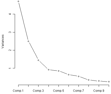
The most obvious change in slope in the scree plot occurs at component 4, which is the “elbow” of the scree plot. Therefore, it cound be argued based on the basis of the scree plot that the first three components should be retained.
Another way of deciding how many components to retain is to use Kaiser’s criterion: that we should only retain principal components for which the variance is above 1 (when principal component analysis was applied to standardised data). We can check this by finding the variance of each of the principal components:
> (wine.pca$sdev)^2
  [1] 4.7058503 2.4969737 1.4460720 0.9189739 0.8532282 0.6416570 0.5510283 0.3484974
  [9] 0.2888799 0.2509025 0.2257886 0.1687702 0.1033779
We see that the variance is above 1 for principal components 1, 2, and 3 (which have variances 4.71, 2.50, and 1.45, respectively). Therefore, using Kaiser’s criterion, we would retain the first three principal components.
A third way to decide how many principal components to retain is to decide to keep the number of components required to explain at least some minimum amount of the total variance. For example, if it is important to explain at least 80% of the variance, we would retain the first five principal components, as we can see from the output of “summary(wine.pca)” that the first five principal components explain 80.2% of the variance (while the first four components explain just 73.6%, so are not sufficient).
Loadings for the Principal Components
The loadings for the principal components are stored in a named element “rotation” of the variable returned by “prcomp()”. This contains a matrix with the loadings of each principal component, where the first column in the matrix contains the loadings for the first principal component, the second column contains the loadings for the second principal component, and so on.
Therefore, to obtain the loadings for the first principal component in our analysis of the 13 chemical concentrations in wine samples, we type:
> wine.pca$rotation[,1]
      V2           V3           V4           V5           V6           V7
  -0.144329395  0.245187580  0.002051061  0.239320405 -0.141992042 -0.394660845
      V8           V9          V10          V11          V12          V13
  -0.422934297  0.298533103 -0.313429488  0.088616705 -0.296714564 -0.376167411
     V14
  -0.286752227
This means that the first principal component is a linear combination of the variables: -0.144*Z2 + 0.245*Z3 + 0.002*Z4 + 0.239*Z5 - 0.142*Z6 - 0.395*Z7 - 0.423*Z8 + 0.299*Z9 -0.313*Z10 + 0.089*Z11 - 0.297*Z12 - 0.376*Z13 - 0.287*Z14, where Z2, Z3, Z4...Z14 are the standardised versions of the variables V2, V3, V4...V14 (that each have mean of 0 and variance of 1).
Note that the square of the loadings sum to 1, as this is a constraint used in calculating the loadings:
> sum((wine.pca$rotation[,1])^2)
  [1] 1
To calculate the values of the first principal component, we can define our own function to calculate a principal component given the loadings and the input variables’ values:
> calcpc <- function(variables,loadings)
  {
     # find the number of samples in the data set
     as.data.frame(variables)
     numsamples <- nrow(variables)
     # make a vector to store the component
     pc <- numeric(numsamples)
     # find the number of variables
     numvariables <- length(variables)
     # calculate the value of the component for each sample
     for (i in 1:numsamples)
     {
        valuei <- 0
        for (j in 1:numvariables)
        {
           valueij <- variables[i,j]
           loadingj <- loadings[j]
           valuei <- valuei + (valueij * loadingj)
        }
        pc[i] <- valuei
     }
     return(pc)
  }
We can then use the function to calculate the values of the first principal component for each sample in our wine data:
> calcpc(standardisedconcentrations, wine.pca$rotation[,1])
  [1] -3.30742097 -2.20324981 -2.50966069 -3.74649719 -1.00607049 -3.04167373 -2.44220051
  [8] -2.05364379 -2.50381135 -2.74588238 -3.46994837 -1.74981688 -2.10751729 -3.44842921
  [15] -4.30065228 -2.29870383 -2.16584568 -1.89362947 -3.53202167 -2.07865856 -3.11561376
  [22] -1.08351361 -2.52809263 -1.64036108 -1.75662066 -0.98729406 -1.77028387 -1.23194878
  [29] -2.18225047 -2.24976267 -2.49318704 -2.66987964 -1.62399801 -1.89733870 -1.40642118
  [36] -1.89847087 -1.38096669 -1.11905070 -1.49796891 -2.52268490 -2.58081526 -0.66660159
  ...
In fact, the values of the first principal component are stored in the variable wine.pca$x[,1] that was returned by the “prcomp()” function, so we can compare those values to the ones that we calculated, and they should agree:
> wine.pca$x[,1]
  [1] -3.30742097 -2.20324981 -2.50966069 -3.74649719 -1.00607049 -3.04167373 -2.44220051
  [8] -2.05364379 -2.50381135 -2.74588238 -3.46994837 -1.74981688 -2.10751729 -3.44842921
  [15] -4.30065228 -2.29870383 -2.16584568 -1.89362947 -3.53202167 -2.07865856 -3.11561376
  [22] -1.08351361 -2.52809263 -1.64036108 -1.75662066 -0.98729406 -1.77028387 -1.23194878
  [29] -2.18225047 -2.24976267 -2.49318704 -2.66987964 -1.62399801 -1.89733870 -1.40642118
  [36] -1.89847087 -1.38096669 -1.11905070 -1.49796891 -2.52268490 -2.58081526 -0.66660159
  ...
We see that they do agree.
The first principal component has highest (in absolute value) loadings for V8 (-0.423), V7 (-0.395), V13 (-0.376), V10 (-0.313), V12 (-0.297), V14 (-0.287), V9 (0.299), V3 (0.245), and V5 (0.239). The loadings for V8, V7, V13, V10, V12 and V14 are negative, while those for V9, V3, and V5 are positive. Therefore, an interpretation of the first principal component is that it represents a contrast between the concentrations of V8, V7, V13, V10, V12, and V14, and the concentrations of V9, V3 and V5.
Similarly, we can obtain the loadings for the second principal component by typing:
> wine.pca$rotation[,2]
      V2           V3           V4           V5           V6           V7
  0.483651548  0.224930935  0.316068814 -0.010590502  0.299634003  0.065039512
      V8           V9          V10          V11          V12          V13
  -0.003359812  0.028779488  0.039301722  0.529995672 -0.279235148 -0.164496193
     V14
  0.364902832
This means that the second principal component is a linear combination of the variables: 0.484*Z2 + 0.225*Z3 + 0.316*Z4 - 0.011*Z5 + 0.300*Z6 + 0.065*Z7 - 0.003*Z8 + 0.029*Z9 + 0.039*Z10 + 0.530*Z11 - 0.279*Z12 - 0.164*Z13 + 0.365*Z14, where Z1, Z2, Z3...Z14 are the standardised versions of variables V2, V3, ... V14 that each have mean 0 and variance 1.
Note that the square of the loadings sum to 1, as above:
> sum((wine.pca$rotation[,2])^2)
  [1] 1
The second principal component has highest loadings for V11 (0.530), V2 (0.484), V14 (0.365), V4 (0.316), V6 (0.300), V12 (-0.279), and V3 (0.225). The loadings for V11, V2, V14, V4, V6 and V3 are positive, while the loading for V12 is negative. Therefore, an interpretation of the second principal component is that it represents a contrast between the concentrations of V11, V2, V14, V4, V6 and V3, and the concentration of V12. Note that the loadings for V11 (0.530) and V2 (0.484) are the largest, so the contrast is mainly between the concentrations of V11 and V2, and the concentration of V12.
Scatterplots of the Principal Components
The values of the principal components are stored in a named element “x” of the variable returned by “prcomp()”. This contains a matrix with the principal components, where the first column in the matrix contains the first principal component, the second column the second component, and so on.
Thus, in our example, “wine.pca$x[,1]” contains the first principal component, and “wine.pca$x[,2]” contains the second principal component.
We can make a scatterplot of the first two principal components, and label the data points with the cultivar that the wine samples come from, by typing:
> plot(wine.pca$x[,1],wine.pca$x[,2]) # make a scatterplot
> text(wine.pca$x[,1],wine.pca$x[,2], wine$V1, cex=0.7, pos=4, col="red") # add labels

The scatterplot shows the first principal component on the x-axis, and the second principal component on the y-axis. We can see from the scatterplot that wine samples of cultivar 1 have much lower values of the first principal component than wine samples of cultivar 3. Therefore, the first principal component separates wine samples of cultivars 1 from those of cultivar 3.
We can also see that wine samples of cultivar 2 have much higher values of the second principal component than wine samples of cultivars 1 and 3. Therefore, the second principal component separates samples of cultivar 2 from samples of cultivars 1 and 3.
Therefore, the first two principal components are reasonably useful for distinguishing wine samples of the three different cultivars.
Above, we interpreted the first principal component as a contrast between the concentrations of V8, V7, V13, V10, V12, and V14, and the concentrations of V9, V3 and V5. We can check whether this makes sense in terms of the concentrations of these chemicals in the different cultivars, by printing out the means of the standardised concentration variables in each cultivar, using the “printMeanAndSdByGroup()” function (see above):
> printMeanAndSdByGroup(standardisedconcentrations,wine[1])
  [1] "Means:"
    V1         V2         V3         V4         V5          V6          V7          V8          V9        V10        V11        V12        V13        V14
  1  1  0.9166093 -0.2915199  0.3246886 -0.7359212  0.46192317  0.87090552  0.95419225 -0.57735640  0.5388633  0.2028288  0.4575567  0.7691811  1.1711967
  2  2 -0.8892116 -0.3613424 -0.4437061  0.2225094 -0.36354162 -0.05790375  0.05163434  0.01452785  0.0688079 -0.8503999  0.4323908  0.2446043 -0.7220731
  3  3  0.1886265  0.8928122  0.2572190  0.5754413 -0.03004191 -0.98483874 -1.24923710  0.68817813 -0.7641311  1.0085728 -1.2019916 -1.3072623 -0.3715295
Does it make sense that the first principal component can separate cultivar 1 from cultivar 3? In cultivar 1, the mean values of V8 (0.954), V7 (0.871), V13 (0.769), V10 (0.539), V12 (0.458) and V14 (1.171) are very high compared to the mean values of V9 (-0.577), V3 (-0.292) and V5 (-0.736). In cultivar 3, the mean values of V8 (-1.249), V7 (-0.985), V13 (-1.307), V10 (-0.764), V12 (-1.202) and V14 (-0.372) are very low compared to the mean values of V9 (0.688), V3 (0.893) and V5 (0.575). Therefore, it does make sense that principal component 1 is a contrast between the concentrations of V8, V7, V13, V10, V12, and V14, and the concentrations of V9, V3 and V5; and that principal component 1 can separate cultivar 1 from cultivar 3.
Above, we intepreted the second principal component as a contrast between the concentrations of V11, V2, V14, V4, V6 and V3, and the concentration of V12. In the light of the mean values of these variables in the different cultivars, does it make sense that the second principal component can separate cultivar 2 from cultivars 1 and 3? In cultivar 1, the mean values of V11 (0.203), V2 (0.917), V14 (1.171), V4 (0.325), V6 (0.462) and V3 (-0.292) are not very different from the mean value of V12 (0.458). In cultivar 3, the mean values of V11 (1.009), V2 (0.189), V14 (-0.372), V4 (0.257), V6 (-0.030) and V3 (0.893) are also not very different from the mean value of V12 (-1.202). In contrast, in cultivar 2, the mean values of V11 (-0.850), V2 (-0.889), V14 (-0.722), V4 (-0.444), V6 (-0.364) and V3 (-0.361) are much less than the mean value of V12 (0.432). Therefore, it makes sense that principal component is a contrast between the concentrations of V11, V2, V14, V4, V6 and V3, and the concentration of V12; and that principal component 2 can separate cultivar 2 from cultivars 1 and 3.
Linear Discriminant Analysis
The purpose of principal component analysis is to find the best low-dimensional representation of the variation in a multivariate data set. For example, in the wine data set, we have 13 chemical concentrations describing wine samples from three cultivars. By carrying out a principal component analysis, we found that most of the variation in the chemical concentrations between the samples can be captured using the first two principal components, where each of the principal components is a particular linear combination of the 13 chemical concentrations.
The purpose of linear discriminant analysis (LDA) is to find the linear combinations of the original variables (the 13 chemical concentrations here) that gives the best possible separation between the groups (wine cultivars here) in our data set. Linear discriminant analysis is also known as “canonical discriminant analysis”, or simply “discriminant analysis”.
If we want to separate the wines by cultivar, the wines come from three different cultivars, so the number of groups (G) is 3, and the number of variables is 13 (13 chemicals’ concentrations; p = 13). The maximum number of useful discriminant functions that can separate the wines by cultivar is the minimum of G-1 and p, and so in this case it is the minimum of 2 and 13, which is 2. Thus, we can find at most 2 useful discriminant functions to separate the wines by cultivar, using the 13 chemical concentration variables.
You can carry out a linear discriminant analysis using the “lda()” function from the R “MASS” package. To use this function, we first need to install the “MASS” R package (for instructions on how to install an R package, see How to install an R package).
For example, to carry out a linear discriminant analysis using the 13 chemical concentrations in the wine samples, we type:
> library("MASS")                                                # load the MASS package
> wine.lda <- lda(wine$V1 ~ wine$V2 + wine$V3 + wine$V4 + wine$V5 + wine$V6 + wine$V7 +
                            wine$V8 + wine$V9 + wine$V10 + wine$V11 + wine$V12 + wine$V13 +
                            wine$V14)
Loadings for the Discriminant Functions
To get the values of the loadings of the discriminant functions for the wine data, we can type:
> wine.lda
  Coefficients of linear discriminants:
              LD1           LD2
  wine$V2  -0.403399781  0.8717930699
  wine$V3   0.165254596  0.3053797325
  wine$V4  -0.369075256  2.3458497486
  wine$V5   0.154797889 -0.1463807654
  wine$V6  -0.002163496 -0.0004627565
  wine$V7   0.618052068 -0.0322128171
  wine$V8  -1.661191235 -0.4919980543
  wine$V9  -1.495818440 -1.6309537953
  wine$V10  0.134092628 -0.3070875776
  wine$V11  0.355055710  0.2532306865
  wine$V12 -0.818036073 -1.5156344987
  wine$V13 -1.157559376  0.0511839665
  wine$V14 -0.002691206  0.0028529846
This means that the first discriminant function is a linear combination of the variables: -0.403*V2 + 0.165*V3 - 0.369*V4 + 0.155*V5 - 0.002*V6 + 0.618*V7 - 1.661*V8 - 1.496*V9 + 0.134*V10 + 0.355*V11 - 0.818*V12 - 1.158*V13 - 0.003*V14, where V2, V3, ... V14 are the concentrations of the 14 chemicals found in the wine samples. For convenience, the value for each discriminant function (eg. the first discriminant function) are scaled so that their mean value is zero (see below).
Note that these loadings are calculated so that the within-group variance of each discriminant function for each group (cultivar) is equal to 1, as will be demonstrated below.
These scalings are also stored in the named element “scaling” of the variable returned by the lda() function. This element contains a matrix, in which the first column contains the loadings for the first discriminant function, the second column contains the loadings for the second discriminant function and so on. For example, to extract the loadings for the first discriminant function, we can type:
> wine.lda$scaling[,1]
   wine$V2      wine$V3      wine$V4      wine$V5      wine$V6      wine$V7
 -0.403399781  0.165254596 -0.369075256  0.154797889 -0.002163496  0.618052068
   wine$V8      wine$V9     wine$V10     wine$V11     wine$V12     wine$V13
 -1.661191235 -1.495818440  0.134092628  0.355055710 -0.818036073 -1.157559376
  wine$V14
 -0.002691206
To calculate the values of the first discriminant function, we can define our own function “calclda()”:
> calclda <- function(variables,loadings)
  {
     # find the number of samples in the data set
     as.data.frame(variables)
     numsamples <- nrow(variables)
     # make a vector to store the discriminant function
     ld <- numeric(numsamples)
     # find the number of variables
     numvariables <- length(variables)
     # calculate the value of the discriminant function for each sample
     for (i in 1:numsamples)
     {
        valuei <- 0
        for (j in 1:numvariables)
        {
           valueij <- variables[i,j]
           loadingj <- loadings[j]
           valuei <- valuei + (valueij * loadingj)
        }
        ld[i] <- valuei
     }
     # standardise the discriminant function so that its mean value is 0:
     ld <- as.data.frame(scale(ld, center=TRUE, scale=FALSE))
     ld <- ld[[1]]
     return(ld)
  }
The function calclda() simply calculates the value of a discriminant function for each sample in the data set, for example, for the first disriminant function, for each sample we calculate the value using the equation -0.403*V2 - 0.165*V3 - 0.369*V4 + 0.155*V5 - 0.002*V6 + 0.618*V7 - 1.661*V8 - 1.496*V9 + 0.134*V10 + 0.355*V11 - 0.818*V12 - 1.158*V13 - 0.003*V14. Furthermore, the “scale()” command is used within the calclda() function in order to standardise the value of a discriminant function (eg. the first discriminant function) so that its mean value (over all the wine samples) is 0.
We can use the function calclda() to calculate the values of the first discriminant function for each sample in our wine data:
> calclda(wine[2:14], wine.lda$scaling[,1])
  [1] -4.70024401 -4.30195811 -3.42071952 -4.20575366 -1.50998168 -4.51868934
  [7] -4.52737794 -4.14834781 -3.86082876 -3.36662444 -4.80587907 -3.42807646
  [13] -3.66610246 -5.58824635 -5.50131449 -3.18475189 -3.28936988 -2.99809262
  [19] -5.24640372 -3.13653106 -3.57747791 -1.69077135 -4.83515033 -3.09588961
  [25] -3.32164716 -2.14482223 -3.98242850 -2.68591432 -3.56309464 -3.17301573
  [31] -2.99626797 -3.56866244 -3.38506383 -3.52753750 -2.85190852 -2.79411996
  ...
In fact, the values of the first linear discriminant function can be calculated using the “predict()” function in R, so we can compare those to the ones that we calculated, and they should agree:
> wine.lda.values <- predict(wine.lda, wine[2:14])
> wine.lda.values$x[,1] # contains the values for the first discriminant function
      1           2           3           4           5           6
  -4.70024401 -4.30195811 -3.42071952 -4.20575366 -1.50998168 -4.51868934
      7           8           9          10          11          12
  -4.52737794 -4.14834781 -3.86082876 -3.36662444 -4.80587907 -3.42807646
     13          14          15          16          17          18
  -3.66610246 -5.58824635 -5.50131449 -3.18475189 -3.28936988 -2.99809262
     19          20          21          22          23          24
  -5.24640372 -3.13653106 -3.57747791 -1.69077135 -4.83515033 -3.09588961
     25          26          27          28          29          30
  -3.32164716 -2.14482223 -3.98242850 -2.68591432 -3.56309464 -3.17301573
     31          32          33          34          35          36
  -2.99626797 -3.56866244 -3.38506383 -3.52753750 -2.85190852 -2.79411996
  ...
We see that they do agree.
It doesn’t matter whether the input variables for linear discriminant analysis are standardised or not, unlike for principal components analysis in which it is often necessary to standardise the input variables. However, using standardised variables in linear discriminant analysis makes it easier to interpret the loadings in a linear discriminant function.
In linear discriminant analysis, the standardised version of an input variable is defined so that it has mean zero and within-groups variance of 1. Thus, we can calculate the “group-standardised” variable by subtracting the mean from each value of the variable, and dividing by the within-groups standard deviation. To calculate the group-standardised version of a set of variables, we can use the function “groupStandardise()” below:
> groupStandardise <- function(variables, groupvariable)
  {
     # find out how many variables we have
     variables <- as.data.frame(variables)
     numvariables <- length(variables)
     # find the variable names
     variablenames <- colnames(variables)
     # calculate the group-standardised version of each variable
     for (i in 1:numvariables)
     {
        variablei <- variables[i]
        variablei_name <- variablenames[i]
        variablei_Vw <- calcWithinGroupsVariance(variablei, groupvariable)
        variablei_mean <- mean(variablei)
        variablei_new <- (variablei - variablei_mean)/(sqrt(variablei_Vw))
        data_length <- nrow(variablei)
        if (i == 1) { variables_new <- data.frame(row.names=seq(1,data_length)) }
        variables_new[`variablei_name`] <- variablei_new
     }
     return(variables_new)
  }
For example, we can use the “groupStandardise()” function to calculate the group-standardised versions of the chemical concentrations in wine samples:
> groupstandardisedconcentrations <- groupStandardise(wine[2:14], wine[1])
We can then use the lda() function to perform linear disriminant analysis on the group-standardised variables:
> wine.lda2 <- lda(wine$V1 ~ groupstandardisedconcentrations$V2 + groupstandardisedconcentrations$V3 +
                             groupstandardisedconcentrations$V4 + groupstandardisedconcentrations$V5 +
                             groupstandardisedconcentrations$V6 + groupstandardisedconcentrations$V7 +
                             groupstandardisedconcentrations$V8 + groupstandardisedconcentrations$V9 +
                             groupstandardisedconcentrations$V10 + groupstandardisedconcentrations$V11 +
                             groupstandardisedconcentrations$V12 + groupstandardisedconcentrations$V13 +
                             groupstandardisedconcentrations$V14)
> wine.lda2
  Coefficients of linear discriminants:
                                            LD1          LD2
  groupstandardisedconcentrations$V2  -0.20650463  0.446280119
  groupstandardisedconcentrations$V3   0.15568586  0.287697336
  groupstandardisedconcentrations$V4  -0.09486893  0.602988809
  groupstandardisedconcentrations$V5   0.43802089 -0.414203541
  groupstandardisedconcentrations$V6  -0.02907934 -0.006219863
  groupstandardisedconcentrations$V7   0.27030186 -0.014088108
  groupstandardisedconcentrations$V8  -0.87067265 -0.257868714
  groupstandardisedconcentrations$V9  -0.16325474 -0.178003512
  groupstandardisedconcentrations$V10  0.06653116 -0.152364015
  groupstandardisedconcentrations$V11  0.53670086  0.382782544
  groupstandardisedconcentrations$V12 -0.12801061 -0.237174509
  groupstandardisedconcentrations$V13 -0.46414916  0.020523349
  groupstandardisedconcentrations$V14 -0.46385409  0.491738050
It makes sense to interpret the loadings calculated using the group-standardised variables rather than the loadings for the original (unstandardised) variables.
In the first discriminant function calculated for the group-standardised variables, the largest loadings (in absolute) value are given to V8 (-0.871), V11 (0.537), V13 (-0.464), V14 (-0.464), and V5 (0.438). The loadings for V8, V13 and V14 are negative, while those for V11 and V5 are positive. Therefore, the discriminant function seems to represent a contrast between the concentrations of V8, V13 and V14, and the concentrations of V11 and V5.
We saw above that the individual variables which gave the greatest separations between the groups were V8 (separation 233.93), V14 (207.92), V13 (189.97), V2 (135.08) and V11 (120.66). These were mostly the same variables that had the largest loadings in the linear discriminant function (loading for V8: -0.871, for V14: -0.464, for V13: -0.464, for V11: 0.537).
We found above that variables V8 and V11 have a negative between-groups covariance (-60.41) and a positive within-groups covariance (0.29). When the between-groups covariance and within-groups covariance for two variables have opposite signs, it indicates that a better separation between groups can be obtained by using a linear combination of those two variables than by using either variable on its own.
Thus, given that the two variables V8 and V11 have between-groups and within-groups covariances of opposite signs, and that these are two of the variables that gave the greatest separations between groups when used individually, it is not surprising that these are the two variables that have the largest loadings in the first discriminant function.
Note that although the loadings for the group-standardised variables are easier to interpret than the loadings for the unstandardised variables, the values of the discriminant function are the same regardless of whether we standardise the input variables or not. For example, for wine data, we can calculate the value of the first discriminant function calculated using the unstandardised and group-standardised variables by typing:
> wine.lda.values <- predict(wine.lda, wine[2:14])
> wine.lda.values$x[,1] # values for the first discriminant function, using the unstandardised data
      1           2           3           4           5           6
  -4.70024401 -4.30195811 -3.42071952 -4.20575366 -1.50998168 -4.51868934
      7           8           9          10          11          12
  -4.52737794 -4.14834781 -3.86082876 -3.36662444 -4.80587907 -3.42807646
     13          14          15          16          17          18
  -3.66610246 -5.58824635 -5.50131449 -3.18475189 -3.28936988 -2.99809262
     19          20          21          22          23          24
  -5.24640372 -3.13653106 -3.57747791 -1.69077135 -4.83515033 -3.09588961
  ...
> wine.lda.values2 <- predict(wine.lda2, groupstandardisedconcentrations)
> wine.lda.values2$x[,1] # values for the first discriminant function, using the standardised data
      1           2           3           4           5           6
  -4.70024401 -4.30195811 -3.42071952 -4.20575366 -1.50998168 -4.51868934
      7           8           9          10          11          12
  -4.52737794 -4.14834781 -3.86082876 -3.36662444 -4.80587907 -3.42807646
     13          14          15          16          17          18
  -3.66610246 -5.58824635 -5.50131449 -3.18475189 -3.28936988 -2.99809262
     19          20          21          22          23          24
  -5.24640372 -3.13653106 -3.57747791 -1.69077135 -4.83515033 -3.09588961
  ...
We can see that although the loadings are different for the first discriminant functions calculated using unstandardised and group-standardised data, the actual values of the first discriminant function are the same.
Separation Achieved by the Discriminant Functions
To calculate the separation achieved by each discriminant function, we first need to calculate the value of each discriminant function, by substituting the variables’ values into the linear combination for the discriminant function (eg. -0.403*V2 - 0.165*V3 - 0.369*V4 + 0.155*V5 - 0.002*V6 + 0.618*V7 - 1.661*V8 - 1.496*V9 + 0.134*V10 + 0.355*V11 - 0.818*V12 - 1.158*V13 - 0.003*V14 for the first discriminant function), and then scaling the values of the discriminant function so that their mean is zero.
As mentioned above, we can do this using the “predict()” function in R. For example, to calculate the value of the discriminant functions for the wine data, we type:
> wine.lda.values <- predict(wine.lda, standardisedconcentrations)
The returned variable has a named element “x” which is a matrix containing the linear discriminant functions: the first column of x contains the first discriminant function, the second column of x contains the second discriminant function, and so on (if there are more discriminant functions).
We can therefore calculate the separations achieved by the two linear discriminant functions for the wine data by using the “calcSeparations()” function (see above), which calculates the separation as the ratio of the between-groups variance to the within-groups variance:
> calcSeparations(wine.lda.values$x,wine[1])
  [1] "variable LD1 Vw= 1 Vb= 794.652200566216 separation= 794.652200566216"
  [1] "variable LD2 Vw= 1 Vb= 361.241041493455 separation= 361.241041493455"
As mentioned above, the loadings for each discriminant function are calculated in such a way that the within-group variance (Vw) for each group (wine cultivar here) is equal to 1, as we see in the output from calcSeparations() above.
The output from calcSeparations() tells us that the separation achieved by the first (best) discriminant function is 794.7, and the separation achieved by the second (second best) discriminant function is 361.2.
Therefore, the total separation is the sum of these, which is (794.652200566216+361.241041493455=1155.893) 1155.89, rounded to two decimal places. Therefore, the “percentage separation” achieved by the first discriminant function is (794.652200566216*100/1155.893=) 68.75%, and the percentage separation achieved by the second discriminant function is (361.241041493455*100/1155.893=) 31.25%.
The “proportion of trace” that is printed when you type “wine.lda” (the variable returned by the lda() function) is the percentage separation achieved by each discriminant function. For example, for the wine data we get the same values as just calculated (68.75% and 31.25%):
> wine.lda
  Proportion of trace:
    LD1    LD2
  0.6875 0.3125
Therefore, the first discriminant function does achieve a good separation between the three groups (three cultivars), but the second discriminant function does improve the separation of the groups by quite a large amount, so is it worth using the second discriminant function as well. Therefore, to achieve a good separation of the groups (cultivars), it is necessary to use both of the first two discriminant functions.
We found above that the largest separation achieved for any of the individual variables (individual chemical concentrations) was 233.9 for V8, which is quite a lot less than 794.7, the separation achieved by the first discriminant function. Therefore, the effect of using more than one variable to calculate the discriminant function is that we can find a discriminant function that achieves a far greater separation between groups than achieved by any one variable alone.
The variable returned by the lda() function also has a named element “svd”, which contains the ratio of between- and within-group standard deviations for the linear discriminant variables, that is, the square root of the “separation” value that we calculated using calcSeparations() above. When we calculate the square of the value stored in “svd”, we should get the same value as found using calcSeparations():
> (wine.lda$svd)^2
  [1] 794.6522 361.2410
A Stacked Histogram of the LDA Values
A nice way of displaying the results of a linear discriminant analysis (LDA) is to make a stacked histogram of the values of the discriminant function for the samples from different groups (different wine cultivars in our example).
We can do this using the “ldahist()” function in R. For example, to make a stacked histogram of the first discriminant function’s values for wine samples of the three different wine cultivars, we type:
> ldahist(data = wine.lda.values$x[,1], g=wine$V1)
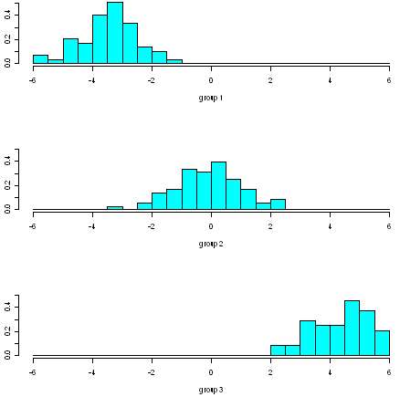
We can see from the histogram that cultivars 1 and 3 are well separated by the first discriminant function, since the values for the first cultivar are between -6 and -1, while the values for cultivar 3 are between 2 and 6, and so there is no overlap in values.
However, the separation achieved by the linear discriminant function on the training set may be an overestimate. To get a more accurate idea of how well the first discriminant function separates the groups, we would need to see a stacked histogram of the values for the three cultivars using some unseen “test set”, that is, using a set of data that was not used to calculate the linear discriminant function.
We see that the first discriminant function separates cultivars 1 and 3 very well, but does not separate cultivars 1 and 2, or cultivars 2 and 3, so well.
We therefore investigate whether the second discriminant function separates those cultivars, by making a stacked histogram of the second discriminant function’s values:
> ldahist(data = wine.lda.values$x[,2], g=wine$V1)
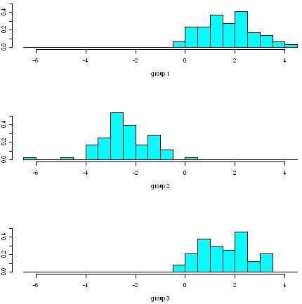
We see that the second discriminant function separates cultivars 1 and 2 quite well, although there is a little overlap in their values. Furthermore, the second discriminant function also separates cultivars 2 and 3 quite well, although again there is a little overlap in their values so it is not perfect.
Thus, we see that two discriminant functions are necessary to separate the cultivars, as was discussed above (see the discussion of percentage separation above).
Scatterplots of the Discriminant Functions
We can obtain a scatterplot of the best two discriminant functions, with the data points labelled by cultivar, by typing:
> plot(wine.lda.values$x[,1],wine.lda.values$x[,2]) # make a scatterplot
> text(wine.lda.values$x[,1],wine.lda.values$x[,2],wine$V1,cex=0.7,pos=4,col="red") # add labels
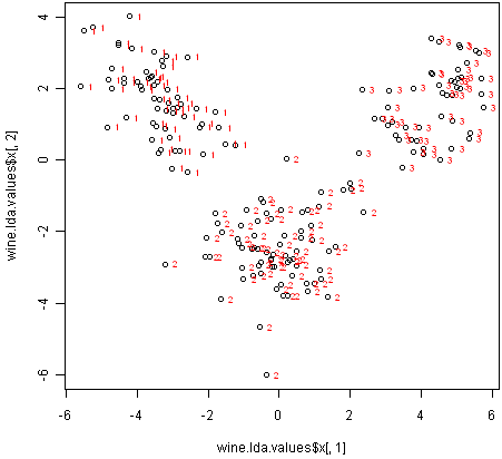
From the scatterplot of the first two discriminant functions, we can see that the wines from the three cultivars are well separated in the scatterplot. The first discriminant function (x-axis) separates cultivars 1 and 3 very well, but doesn’t not perfectly separate cultivars 1 and 3, or cultivars 2 and 3.
The second discriminant function (y-axis) achieves a fairly good separation of cultivars 1 and 3, and cultivars 2 and 3, although it is not totally perfect.
To achieve a very good separation of the three cultivars, it would be best to use both the first and second discriminant functions together, since the first discriminant function can separate cultivars 1 and 3 very well, and the second discriminant function can separate cultivars 1 and 2, and cultivars 2 and 3, reasonably well.
Allocation Rules and Misclassification Rate
We can calculate the mean values of the discriminant functions for each of the three cultivars using the “printMeanAndSdByGroup()” function (see above):
> printMeanAndSdByGroup(wine.lda.values$x,wine[1])
  [1] "Means:"
     V1         LD1       LD2
   1  1 -3.42248851  1.691674
   2  2 -0.07972623 -2.472656
   3  3  4.32473717  1.578120
We find that the mean value of the first discriminant function is -3.42248851 for cultivar 1, -0.07972623 for cultivar 2, and 4.32473717 for cultivar 3. The mid-way point between the mean values for cultivars 1 and 2 is (-3.42248851-0.07972623)/2=-1.751107, and the mid-way point between the mean values for cultivars 2 and 3 is (-0.07972623+4.32473717)/2 = 2.122505.
Therefore, we can use the following allocation rule:
- if the first discriminant function is <= -1.751107, predict the sample to be from cultivar 1
- if the first discriminant function is > -1.751107 and <= 2.122505, predict the sample to be from cultivar 2
- if the first discriminant function is > 2.122505, predict the sample to be from cultivar 3
We can examine the accuracy of this allocation rule by using the “calcAllocationRuleAccuracy()” function below:
> calcAllocationRuleAccuracy <- function(ldavalue, groupvariable, cutoffpoints)
  {
     # find out how many values the group variable can take
     groupvariable2 <- as.factor(groupvariable[[1]])
     levels <- levels(groupvariable2)
     numlevels <- length(levels)
     # calculate the number of true positives and false negatives for each group
     numlevels <- length(levels)
     for (i in 1:numlevels)
     {
        leveli <- levels[i]
        levelidata <- ldavalue[groupvariable==leveli]
        # see how many of the samples from this group are classified in each group
        for (j in 1:numlevels)
        {
           levelj <- levels[j]
           if (j == 1)
           {
              cutoff1 <- cutoffpoints[1]
              cutoff2 <- "NA"
              results <- summary(levelidata <= cutoff1)
           }
           else if (j == numlevels)
           {
              cutoff1 <- cutoffpoints[(numlevels-1)]
              cutoff2 <- "NA"
              results <- summary(levelidata > cutoff1)
           }
           else
           {
              cutoff1 <- cutoffpoints[(j-1)]
              cutoff2 <- cutoffpoints[(j)]
              results <- summary(levelidata > cutoff1 & levelidata <= cutoff2)
           }
           trues <- results["TRUE"]
           trues <- trues[[1]]
           print(paste("Number of samples of group",leveli,"classified as group",levelj," : ",
              trues,"(cutoffs:",cutoff1,",",cutoff2,")"))
        }
     }
  }
For example, to calculate the accuracy for the wine data based on the allocation rule for the first discriminant function, we type:
> calcAllocationRuleAccuracy(wine.lda.values$x[,1], wine[1], c(-1.751107, 2.122505))
  [1] "Number of samples of group 1 classified as group 1  :  56 (cutoffs: -1.751107 , NA )"
  [1] "Number of samples of group 1 classified as group 2  :  3 (cutoffs: -1.751107 , 2.122505 )"
  [1] "Number of samples of group 1 classified as group 3  :  NA (cutoffs: 2.122505 , NA )"
  [1] "Number of samples of group 2 classified as group 1  :  5 (cutoffs: -1.751107 , NA )"
  [1] "Number of samples of group 2 classified as group 2  :  65 (cutoffs: -1.751107 , 2.122505 )"
  [1] "Number of samples of group 2 classified as group 3  :  1 (cutoffs: 2.122505 , NA )"
  [1] "Number of samples of group 3 classified as group 1  :  NA (cutoffs: -1.751107 , NA )"
  [1] "Number of samples of group 3 classified as group 2  :  NA (cutoffs: -1.751107 , 2.122505 )"
  [1] "Number of samples of group 3 classified as group 3  :  48 (cutoffs: 2.122505 , NA )"
This can be displayed in a “confusion matrix”:
| Allocated to group 1 | Allocated to group 2 | Allocated to group 3 | |
|---|---|---|---|
| Is group 1 | 56 | 3 | 0 |
| Is group 2 | 5 | 65 | 1 |
| Is group 3 | 0 | 0 | 48 |
There are 3+5+1=9 wine samples that are misclassified, out of (56+3+5+65+1+48=) 178 wine samples: 3 samples from cultivar 1 are predicted to be from cultivar 2, 5 samples from cultivar 2 are predicted to be from cultivar 1, and 1 sample from cultivar 2 is predicted to be from cultivar 3. Therefore, the misclassification rate is 9/178, or 5.1%. The misclassification rate is quite low, and therefore the accuracy of the allocation rule appears to be relatively high.
However, this is probably an underestimate of the misclassification rate, as the allocation rule was based on this data (this is the “training set”). If we calculated the misclassification rate for a separate “test set” consisting of data other than that used to make the allocation rule, we would probably get a higher estimate of the misclassification rate.
Links and Further Reading
Here are some links for further reading.
For a more in-depth introduction to R, a good online tutorial is available on the “Kickstarting R” website, cran.r-project.org/doc/contrib/Lemon-kickstart.
There is another nice (slightly more in-depth) tutorial to R available on the “Introduction to R” website, cran.r-project.org/doc/manuals/R-intro.html.
To learn about multivariate analysis, I would highly recommend the book “Multivariate analysis” (product code M249/03) by the Open University, available from the Open University Shop.
There is a book available in the “Use R!” series on using R for multivariate analyses, An Introduction to Applied Multivariate Analysis with R by Everitt and Hothorn.
Acknowledgements
Many of the examples in this booklet are inspired by examples in the excellent Open University book, “Multivariate Analysis” (product code M249/03), available from the Open University Shop.
I am grateful to the UCI Machine Learning Repository, http://archive.ics.uci.edu/ml, for making data sets available which I have used in the examples in this booklet.
Thank you to the following users for very helpful comments: to Rich O’Hara and Patrick Hausmann for pointing out that sd(<data.frame>) and mean(<data.frame>) is deprecated; to Arnau Serra-Cayuela for pointing out a typo in the LDA section; to John Christie for suggesting a more compact form for my printMeanAndSdByGroup() function, and to Rama Ramakrishnan for suggesting a more compact form for my mosthighlycorrelated() function.
Contact
I will be grateful if you will send me (Avril Coghlan) corrections or suggestions for improvements to my email address alc@sanger.ac.uk
License
The content in this book is licensed under a Creative Commons Attribution 3.0 License.